When is classical Computer Vision superior to Deep Learning?

‍

All of us have seen great stories of what is possible with Deep Learning (DL). It allows cars to drive on their own, determines the best treatment for patients, and can also put your face into any video clip you like.

Because of the many successes with DL, it only seems natural to apply it to any problem you want to solve. Beware of that bias: Using DL on problems that could be solved with less complex methods creates additional work on costs that you should rather avoid.

In this post I will show you exactly what the advantages and disadvantages of DL are and when it’s best to avoid it completely. Users that are familiar with DL can skip to section Disadvantages of DL to come straight to my arguments.

What is Deep Learning?

To understand the (dis-)advantages of DL, it is important to first gain a general understanding of the process. Simply put, DL describes a process during which a mathematical model learns to produce a desired outcome given large amounts of training data.

The mathematical model in this case is a multi-layered neural network, often containing convolutional and max-pool layers. In practice, you can think of the neural network as many interconnected logistic regressions.

A logistic regression is a function that categorises items given certain measurements. Logistic regressions can be used to determine wether a tissue sample is cancerous or not, e.g. based on cell size, cell shapes, and other measurements. These measurements have to be encoded in numerical data to be processed in the logistic regression.

Similarly, a DL model can determine whether an image contains a cat or not, based on the image data (pixels). To make this possible, the raw pixels are transformed in the multiple layers (e.g. via convolution). You can imagine these layers to contain multiple tests: does the image contain eyes, ears, whiskers: All the features that we would associate with cats (see this blog post for a great visualisation).

Deep Learning needs a lot of training data

To learn which tests it should use, the DL model gets presented with many different images (the training data). At first there are random tests included in the model and with each training step the tests get changed in a way to make the final decision more accurate (this process is called backpropagation).

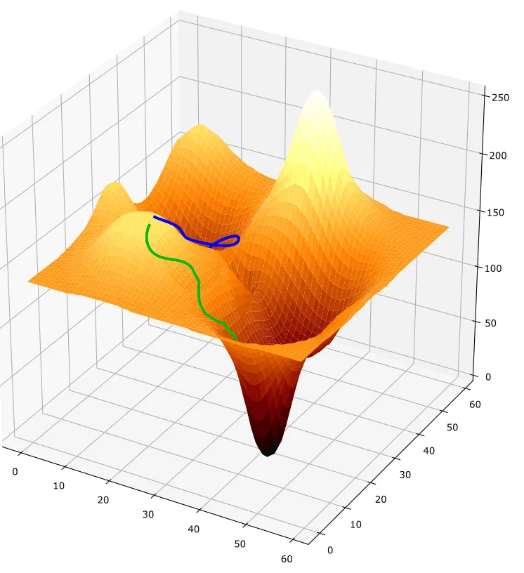
Example for two gradient descent runs. The successful run, reaching the global optimum, is shown in green. The unsuccessful run that gets stuck in a local minimum is shown in blue.

Here we come to the first problem of DL: You need a lot of training data. In case of cat picture this can be quite easy to obtain, but in other cases this can be rather difficult. Also, the training data has to be labelled which can pose an additional challenge.

In addition to the problem of acquiring training data, there are also many quality requirements on the training data. The training data should be as similar as possible to the data the model will be used on. Additionally, there should be no artefacts in the training data. If, for example, all images with cats contain a certain watermark, the model will likely only learn to distinguish cat pictures based on the watermark.

Training can be time consuming - results are not guaranteed

The actual „learning“ process of DL is what I just described as the model being shown many training images and adjusting its „tests“ to make a more accurate prediction. Mathematically, these processes are called backtracking (used by the model finds out where and how the tests are wrong) and gradient decent (used by the model to determine how to change the tests to make better predictions).

You can imagine gradient descent like starting on top of a mountain (making many errors) and trying go down. The model can only look ahead a few meters at a time (by looking at a fraction of the training data). So the model checks which way the slope is going down and simply starts “walking”, re-checking after every step. When every direction from the model’s position is sloping upwards, the model reached its goal: it has found a valley.

Now comes the real problem: You cannot be sure that the model actually found the lowest spot in the landscape! It could be that the model is just stuck at a high valley. Resolving the metaphor, this means the model is still making many mistakes, but can not find a way to become more accurate.

Furthermore, even if the model actually reaches the lowest spot, it will still take it a long time to get there. That is because the model has to look at all of the training data over and over again to determine which way is down.

Also, the learning process is different each time. That is because the model is initialised randomly (the initial tests it uses are random in the beginning). So it could be that you train your model and reach a very low spot (the model has high accuracy). But then when you adjust the training data or the model, in the next training run you might not reach this low spot anymore.

Conclusion: Disadvantages of DL

To summarise the disadvantages of DL:

• You need a lot of curated & annotated training data

• Training takes a lot of time

• Training is non-deterministic, i.e. it can fail for unknown reasons

Now do not get me wrong: DL is great and I love to use it! But I want to advocate for only using DL in cases where it is actually required. If a simpler solution is possible, that should always be the first choice.

In the next section I want to describe an actual use case where we at LoyJoy have replaced an initial DL solution with a much more agile classical computer vision (CV) approach, saving a lot of time and effort.

Problem definition

Here at LoyJoy, we offer loyalty programs for CPG brands (consumer packaged goods) via chatbots. Consumers can redeem unique alphanumeric codes for rewards. Such codes (like “74GH3D7E”) are often printed somewhere outside or inside the packaging. To make redemption more convenient for consumers, we also recognise codes from images that are sent to us via chat. This process makes the consumer’s life really simple: Open our progressive web app, snap a picture and instantly get your reward!

Image caption to test (floating text example)

Example for an Oreo packaging with a loyalty code on the outside.

Initially, we had created a complex DL solution: Since we did not have tens of thousands of packaging images, we artificially generated them ourselves. Then we trained a multi-layer neural network that was able to recognise all characters of the code in one step. Basically the network performed text field recognition, character separation, and character recognition.

While this approach worked quite well, the time spent generating images and training the network were considerable. Additionally, sometimes the network would not train at all, for unknown reasons.

Classical computer vision approach

In a classical CV approach we can not rely on a model that will eventually learn all the steps needed to complete the task at hand. Instead, we have to determine which methods we can use in conjunction to reach our goal.

For our project we first wanted to replace one part of the DL pipeline, namely the text field recognition. Because the location of the text field on the packaging stays the same this is actually a fairly simple task.

We simply needed a method that could recognise the locations of the text field in the target picture to be able to extract it. In CV the elements of a picture are called features. Such features could be any hard edges with strong contrasts, in our case for example the edges of the text field. There are numerous algorithms for feature extraction such as SURF, SIFT, BRIEF, and AKAZE.

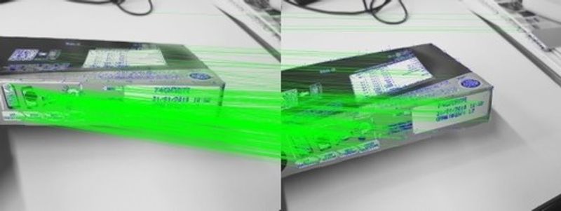
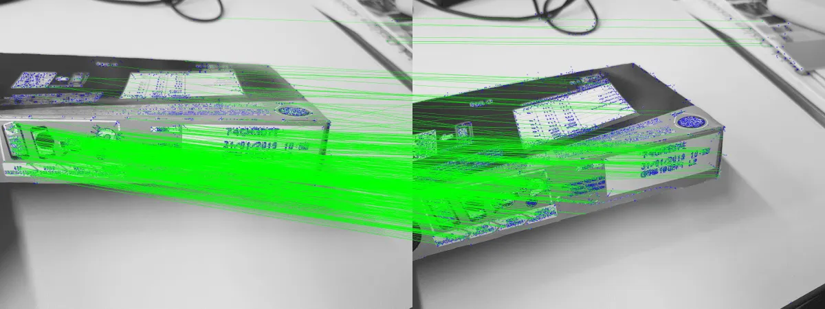
With these edges detected in a reference image of the text field and our target image, we can match the features between the two images and align the target image to the reference image. This matching can be achieved via FLANN or brute force.

Example for matched features between target and reference images. Features are shown as blue circles, green lines indicate matched features.

After matching the features, we can find the homography between the location of the features in the two images. This will basically give us a matrix that describes how we have to transform (turn and distort) the target image to locate the text field in the same location as in the reference image.

Having performed the transformation of the target image, we can simply extract the text field and continue with the optical character recognition step. Here at LoyJoy we continue to use a DL-based system for this step.

Conclusion: Advantages of CV

Using CV for the text field extraction gives us a number of examples in this case:

• We only need one reference image to adapt our system to a new packaging

• We do not have to generate training data

• We do not have to re-train our model

As you can see, the CV model makes our lives quite a bit easier in this case. However, please remember that this case is just one example and that I do not want to advocate only using classical CV all the time.

So, when should we be using classical CV instead of DL? As I said, I would use CV as long as the task is not too complex to be solved using CV. For example, if you want to recognise the same symbol in many different images of similar type, this can be easily done via classical CV.

On the other hand, if you want to recognise various types of objects in all sorts of images, DL is probably the way to go. This can be seen in the ImageNet Large Scale Visual Recognition Challenge (one of the most important CV competitions) where increasingly deep neural networks dominate the winner’s lists.

In the end, there is no obvious solution to the problem. You have to follow your instincts and simply try out different solutions. However, if you suspect that your problem could be solved using classical CV, it is always a good idea to try — implementing a classical CV solution is likely faster than the training of your DL model.